Understanding Big O Notation

When writing software, especially algorithms or data-heavy applications, performance matters. Big O notation is a mathematical way to describe how the runtime or space requirements of an algorithm grow as the input size increases. It helps developers understand how scalable and efficient their code is.

In this post, we'll break down the most common Big O complexities and visualize how they compare as input size increases.

What is Big O Notation?

Big O notation describes the upper bound of an algorithm's growth rate. It gives us a high-level understanding of the algorithm's efficiency by showing how it behaves in the worst-case scenario as the size of the input (n) grows.

Common Time Complexities Compared

Here's a quick overview of common Big O time complexities:

Big O Notation	Name	Example Use Case
O(1)	Constant Time	Accessing a value in an array by index
O(log n)	Logarithmic Time	Binary search
O(n)	Linear Time	Iterating through a list
O(n²)	Quadratic Time	Nested loops (e.g., bubble sort)
O(2^n)	Exponential Time	Recursive algorithms (e.g., Fibonacci)

Time Complexity Comparison Graph

Below is a graph that shows how different time complexities scale as the input size increases:

X-axis: Number of items (n)
**Y-axis: Time (arbitrary units)

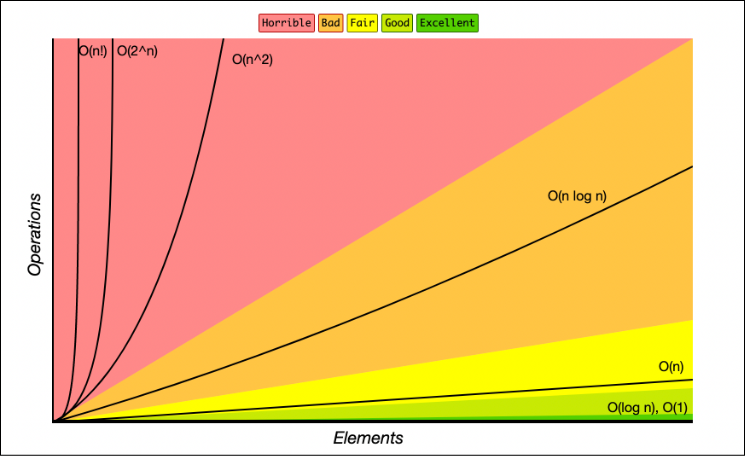
As you can see:

O(1) remains constant regardless of input.
O(log n) grows slowly.
O(n) grows linearly.
O(n²) grows quickly and becomes impractical as n increases.
O(2^n) explodes exponentially and becomes unusable even for small inputs.

Examples

O(1): array[i] – Accessing an index in an array.
O(log n): Binary search on a sorted array.
O(n): Looping through an array to find a value.
O(n²): Comparing every pair in a nested loop.
O(2^n): Recursive solution to the Traveling Salesman Problem.